Bayesian update of a prior normal distribution with new sample information.
The normal distribution.
The probability density function (pdf) is:
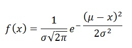
Here x is the variable. It can range from minus infinite to plus infinite.
s is the standard deviation and
m is the mean.
The variance of the mean m is the variance s2 divided by the number of observations.
Updating a distribution
In the updating process it is important to distiguish five different distributions:
Process distribution, the distribution resulting from a data generating process. This is prior information that might be a completely subjective guess, based upon experience that can not be easily tabulated. However, preferably it is based on a collection of data, a sample. For prospect appraisal this is usually a worldwide sampling as used in the Gaeapas appraisal program. Note that for prospect appraisal, the data are almost exclusively mean values of a parameter, such as the mean porosity of a reservoir in a field, not individual porosities in sidewall plugs of pieces of cores.
If the prior is based on a regression analysis, such as API gravity on depth (see below the example), then the process is described as the distribution of the residuals of the regression at a certain "target depth". This distribution has a varying mean and variance along the depth, with the mean following the regression line and the variance dependent on the residual standard deviation and the distance to the mean depth of the data used for the regression. So, each target depth has a (possibly slightly) different distribution.Prior distribution, a distribution obtained from the prior information described above under (1). This distribution is expressing our uncertainty about the mean value of the process. The mean of this prior would be the mean of the process, while the variance would be the process variance divided by the sample size, being the variance of the mean. See also the page on priors.
New information,, a sample of observations of which we calculate a sample mean and a sample variance. It might be sample of size 1, but usually a larger sample. In the case of a world-wide prior (see (2)), the new information may be observations that are local around the prospect to be evaluated, so-called "analogons". It may be clear that, if there is no local information we bring to bear, the best guess is the prior distribution which then can not be updated.
Posterior distribution, the revised, or "updated" prior, based on the sample of new information (3). Note that this distribution is that of the mean. How to go from (2) using (3) to (4) is explained further on this page.
Predictive distribution, the distribution of future observations. This distribution is the one that is used in a Monte Carlo simulation. It combines in the simulation model the world-wide variation of a variable and the relevant local data to give the most realistic value and its uncertainty. The mean of this distribution is the same as the posterior mean, but the variance of this mean is a weighted combination of process and posterior variance. The predictive variance must then still be calculated, invoving the sample size of the process, if available.
I can recommend an explanation of the update process for a probability and for a normal distribution given by Jacobs (2008), which is more complete than what I have given here and explains the derivation of the formulas.
The variables described by the above normal distribution can be porosity, the organic carbon content of a source rock or a recovery efficiency, etc. The World-wide prior distributions we have assembled are distributions of observed values. The bayesian process of obtaining a posterior distribution of observations which can be used for sampling in a Monte Carlo procedure, uses the distribution of the mean of the observations. So the actual prior distribution is telling us how uncertain the mean is. The distribution of this parameter is updated. If we have better than a subjective guess, for instance a worldwide sampling of data, we can estimate the mean and variance of this prior.
When a prior dataset can be roughly represented by a normal distribution, bayesian statistics show that sample information from the same process can be used to obtain a posterior normal distribution. The latter is a weighted combination of the prior and the sample. The larger the sample and the smaller the sample variance, the higher the weight that the sample information receives.
A prior distribution can be constructed by collecting data, or by "subjective experience" which can not be formally processed. In Gaeapas priors are almost exclusively based on world-wide data sets collected from various sources. A subjective element remains however, because it must be decided that the data are relevant, and that the data are independently sampled. In practice a compromise is made that is anyway much better than not using the worldwide background factual experience.
This is especially so, as an appraiser may not have such a wide experience himself. In that sense the baysian update mechanism is similar to what many "expert systems" are providing.
The formulas involved are shown here without giving the derivation (Jacob, 2008, Winkler, 1972). They are valid under the simplifying assumption that we know the "process" variance. This means we can estimate from a world-wide sampling what the variance of the observations is, or subjectively assume such variance.
To get a feel what is behind the math the following reasoning may suffice. In case of no sample information in our local prospect area, all we can do is accept the prior distribution of observations as the "predictive distribution" and use it as input to Gaeapas.
If sample information becomes available it may be that, for instance, a single new measurement "x" will not change our prior estimate when it is equal to the mean of the prior. In that case it has a high likelihood, it "hits" the prior at the highest probability density.
On the other hand, if the new observation is quite far away from the prior mean, the likelihood (density of the prior pdf) is low. In that case we might be tempted to say that in our local prospect area, from which the analog sample information came, the estimation should be different from the prior.
If several new observations are made, the mean value of these is used and compared to the prior distribution. In the following formulas the sample variance is used. By the way, an excellent source to see the math behind the updating procedure, including the treatment of the variance is given by Jacobs, 2008.
The required formulas to obtain the posterior mean (m") and variance (σ"2) under the above assumptions are:
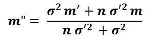
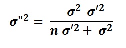
Where m' is the prior mean and m is the sample mean, n the sample size.
For simulation we need the predictive distribution. It has a mean equal to the posterior mean and a standard deviation which we derive from the posterior variance by multiplying with the regression sample size and taking the square root.
Example of an update
The following example of estimating the API gravity (or oil density) may help to see the above formulas at work.
The process mean and variance are derived from a regression of API versus depth. This example is at 3000 m depth, so we have the mean of the process from the regression and the process variance as the square of the (adjusted standard error of estimate, i.e. the variance of the residuals around the regression line. (It could be that the new information samples are not all from 3000m depth, but from betwen 2700 and 3300 meter, say. Then I would use the regression to adjust this data to 3000m depth as if the samples were at equal depth). We obtain the following results when a sample of n, = 8 new density data around our prospect and about at 3000 m depth become available. The mean of the sample is greater than our prior estimate. It is expected that the posterior mean will be larger than the prior. The following data and calculation shows what happens in this example.
| Statistic | Value |
|---|---|
| Depth of estimate - the target | 3000 m |
| Mean of Depth regression | 2135 m |
| The intercept of the regression (beta0) | 22.103 |
| The slope of the regression (beta1) | 0.00425 |
| SE of regression | 7.8165 |
| Adjusted st.deviation residuals | 7.838 |
| Sample size regression | 313 |
| Prior mean m', calculated from the regression at target | 34.85 |
| Prior variance σ'2, from the regression at target | 0.1975 |
| New info; Sample size, n | 8 |
| New info: Sample mean m | 40.56 |
| New info: Sample variance σ2 | 2.67 |
| Posterior mean m" | 36.97 |
| Posterior variance σ"2 | 0.1241 |
| Predictive mean | 36.97 |
| Predictive st.deviation | 6.232 |
In this example an increase of the mean of 6 % is the influence of the 8 new data points. However, the variance is now considerably reduced, or in terms of the standard deviation: from a 7.838 down to 6.232, which is ~80% of the prior st.dev. The first (7.838) would be suggested if only world-wide data are available. If we had a new sample with only 1 new observation (n = 1), and the same sample mean (m) of 40.56, the sample variance (σ2) would be zero. Then we have to resort to taking the same prior variance as the "process", i.e. 0.1975. The posterior mean then becomes 34.99 and the standard deviation 7.765 respectively 0.4% higher and 99% of the prior values. As expected only a small difference.