Correlation and Regression
- Parametric correlation
- Regression equations
- Coefficients
- R-square
- Transformation of variables
- Ortogonal set of independent variables
- Residuals
- Prediction
- t-test and contribution to explained variance
- Autocorrelation
- Causality?
- Outliers
- Rank correlation
- Cross-validation
- Lag-regression
Parametric correlation
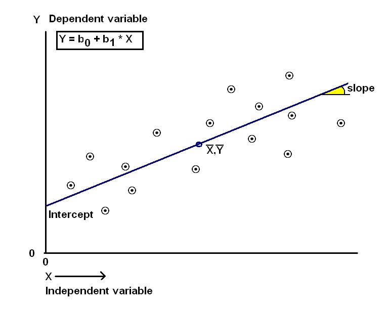
Correlation studies the relationship between two or more variables. Regression uses correlation and estimates a predictive function to relate a dependent variable to an independent one, or a set of independent variables. The regression can be linear or non-linear. Linear regression is provided for in most spreadsheets and performed by a least-squares method. We refer to a very useful textbook on the matter by Edwards (1979).
It is important to stress that correlation does not prove a causal relationship of a pair of variables. In addition an understanding of the data generating processes is required to conclude a causality.
The product-moment correlation coefficient ("r"), in its full glory, is:
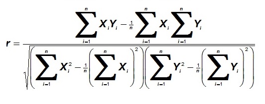
and simple linear regression of a variable Y on X is as in the figure below.
Note that this rather awesome formula dates from the time that we had to do calculations by hand; then first standardizing is extra work. However, in this computer age the equivalent fomula is much simpler if we first "standardize the variables".
The standardized value Y* is:
Y* = (Y - mean of Y)/ standard deviation of Y.
and similar for the X-values. Then the correlation coefficient becomes;
r = Σ(X*1Y*1 + X*2Y*2 .... + X*nY*n)/n
Although for the correlation coefficient it does not matter if we correlate Y on X or X, on Y, the regression of Y on X is not the same as X on Y in the general case. So, for instance, a regression equation of Temperatur vs. depth for estimating temperature, differs from a regression equation, using the same data, for estimating depth from temperature. (However, if standardized variables are used, both regressions are the same and the intercept is zero (regression lines go through the origin). Theoretically you could calculate the one regression equation form the other, by knowing the means and standard deviations of the variables and de-standardizing them in the regression equation).
A few points worth mentioning, in relation to the use of correlation and regression in prospect appraisal, notably GAEAPAS:
Coefficients
A regression equations with 6 independent variables are used by Gaeapas to estimate the HC charge volumes. The coefficients are based on the "calibration set" of well-known accumulations with a worldwide spread. This data is stored in a database of statistical parameters that can be updated, but normally remains unchanged, unless a new calibration is carried out. In this way the experience gained from a sizable geological database is encapsulated in a small set of constants that can be used in a prediction program.
in order to understand the calculation of the multiple regression with matrix algebra, i recommend downloading the Excel worksheet with an excellent complete example (with one independent variable) by Bob Nau from Duke University
The R-square is the fraction of the variance in the regression that is explained by the independent variables. In the calibration carried out by Shell Intl. in the early eighties this was about 0.64, with a samplesize of 160 accumulations and statistically significant. There were 6 X-variables in the regression, representing geological variables of the petroleum system, all individually significant contributors to prediction, and almost totally independent. The dependent variable was the amount of hydrocarbon charge for a prospect (see Sluyk & Nederlof,1984).
- Adjusted R-square.
R-square is always positive. By including ever more X-variables, it will always increase, leading to overly optimistic R-squares. As usually some of the X's do not contribute to the prediction, it is wise to select only the significant contributors. Moreover: calculate the following:
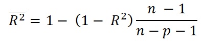
Where p is the number of independent variables.
The effect of this adjustment is large for small samples, but becoming less for increasing n. The result is undefined if n - p < 1. Not surprising as we should always have a sample size n at least one larger than the number of variables for the regression, preferably much larger. Also: the result can become negative if R-square < p / (n-1), reducing the R-square to nothing. If R-square is 1, the adjusted is the same as the original R-square. See also the explanation by Bartlett, J. (2013). The significance of R-square is usually already known from the complete regression results, for instance the t-test on the slope of the regression. If only R-square is known and the number of observations n, and there is only one independent variable, then a value of t can be obtained by the relationship of Pearson's r with t as follows:
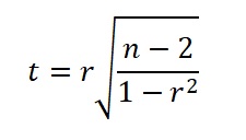
Note: r is the square root of the R-square.
Another possibility is using the Fisher transformation.
- Predicted R-square.
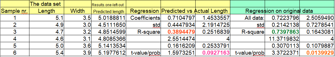
This is one of the possible cross-validation methods. The regression is calculated n times by leaving each time one of the observed data pairs (k) out. Then predict the kth Y-value by the kth regression. By making a new regression of the n predicted values on the n observed Y-values, the predicted R-square is the r-square for that regression.
The following figure is showing results of a calculation on a data set of 6 pairs of values. The important numbers are indicated in different colors. When calculating with all 6 data pairs, the R-square is 0.74, the t-value = 3.37 with 4 d.f. gives a probability of 0.014. However, the predicted R-square is 0.39, t-value 1.60 and the probability 0.093. Such a large effect can be expected when n is so small, but in more usual cases it is an important, sobering reduction of R-square.
The Gaeapas model for HC charge is in principle a multiplication (Sluijk & Nederlof, 1984); therefore the X-variables entering in the product are logtransformed before the regression analysis allowing to use a linear regression model. Although most regression calculations will produce a result, the interpretation may be more difficult. First of all: regression does not prove a causal relationship. Second, one of the requirements of the regression model is that the data are "iid or ("independent and identically distributed"). For time series (also called longitudinal data) this is often not the case, because of autocorrelation in the data. In multiple regression, (several independent X-variables), independence is also often debatable. One of the worst examples is when regression is applied with a variable X as well as X-squared, a parabolic fit. Then the relationship of X and X-squared is causing an inflation in the statistical significance. it works, but interpretation and forecasting must be done very carefully. For a multiple regression the variables are chosen to be as independent as possible. If some of the independent variables would be strongly inter-correlated an ill-conditoned variance/covariance matrix would generate problems for the calculations, but also for the interpretation of the results. When the variables are represented by vectors in space, independent vectors would be perpendicular to each other: "orthogonal".
Residuals are the deviations from the regression line, or the difference between the predicted y-value and the observed. If correlation is perfect (R-square = 1.00/r = 1.00) all the residuals are equal to zero. In practice only the sum of the residuals is zero. The residuals depict the scatter of points around the regression line but the mean of the residuals is zero. If the assumption of , for instance, a linear relationship is valid we would not expect a trend in a plot of residuals in Y versus X. If there is a trend, this would suggest that a linear model is not good enough to describe the relationship. Examples of trends in the residuals are: seasonal variation in a series of monthle data, or a trend suggesting that not only X but also X2 should be included in the model.
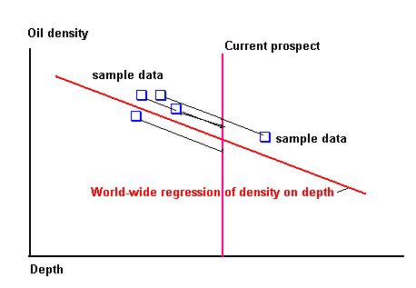
In Gaeapas some of the input variables are correlated with depth. The residuals are a useful tool in prediction and bayesian updating. For instance the API gravity. To combine a worldwide prior for API with local data, the worldwide regression of API on depth is used to find the relevant distribution of residuals at a particular depth. The technique is shown in the following graph.
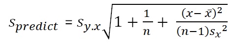
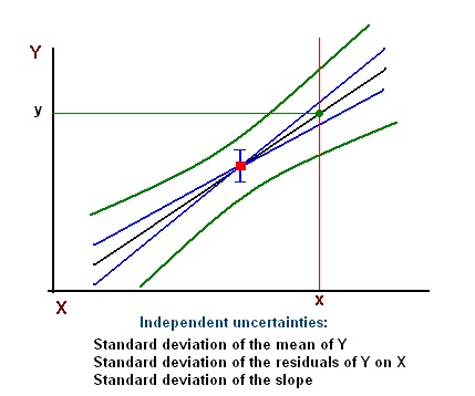
The uncertainties are graphically shown as a formula and as in a figure below. A similar logic holds when there is more than one X-variable.
The following example concerns the regression of condensate ratio (barrels per million cubic feet gas) on reservoir pressure (psia). We have the following regression results:
| Parameter | Value | Number of data points | 73 |
|---|---|
| R-square | 0.455 |
| Intercept, Beta0 | -67.781 |
| Slope, Beta1 | 0.0244 |
| Standard error of estimate ( sy.x) | 69.324 |
| Mean of P | 5250 |
| Variance of P ( sx2) | 6676634 |
| Mean of CGR | 60.37 |
| Variance of CGR | 8744 |
First of all, a prediction of a single value of CGR, given a value of P (x in the above formula) is a draw from a normal distribution with a mean equal to:
and a standard deviation of 69.324, approximately. However, more correct is the standard error of estimate using the formula above.
We use the formula to calculate the standard deviation for the prediction at two values of P. The first at the mean of P and the second in the "outskirts" of P at P = 1000 psia.
| Pressure P | Terms under the root sign | The standard deviation |
|---|---|---|
| 5250 | 1 + 1/73 + (5250 - 5250)^2/(72 * 6676634) = 1.0137 | 1.0068 * 69.324 = 69.795 |
| 1000 | 1 + 1/73 + (1000 - 5250)^2/(72 * 6676634) = 1.0513 | 1.0253 * 69.324 = 71.080 |
Note that the predictive standard deviation at P = 1000 is 2 % larger than at the mean of P. A simulation of the regression would use a routine to create a number of random draws from a standard normal distribution with a mean of zero and a variance of 1. For each P value the associated mean and standard deviation would translate the standard normal deviate in a CGR value. Note that the sample size is larger than 50. This means that the above use of the normal distribution is warranted. If smaller, the t-distribution with n - 1 degrees of freedom would have to be generated instead of the normal, bacause the more exact formula requires that. For our sample size the t-distribution coincides with the normal well enough. This keeps the procedure simpler.
The regression calculation not only gives the values of the coefficients, but also the standard deviations of the coefficients. If the coefficient is zero, it does certainly not contribute to the prediction of Y. Therefore it is useful to see if a beta is significantly different from zero. When we divide a coefficient by its standard deviation we obtain the t-value. Tables of t-values are available for different degrees of freedom, and as a function in spreadsheets. If we assume that the uncertainty of a coefficient is more or less normal, and there are enough degrees of freedom (say > 25), a t-value of 2.0 would already indicate a (mildly) significant coefficient at ~p < 0.05, assuming a two-tailed test. Two-tailed means that you had no idea if the coefficient beta should be negative or positive, and necessarily the same for the t-value. On the contrary if you have assumed a positive beta, a one-tailed test with p < 0.025.
The t-values have another interesting use: The squared t-values of a coefficients are proportional to the part of the R-square associated with it. In other words, squared t-values indicate the relative contributions of the variables to the regression: ANOVA, as the squared t-values are equivalent to the sums of squares in the F-test for significance.
The Least Squares (LS) regression may be strongly influenced by outliers. To get more reliable results, assuming that the outliers can be ignored to a certain extent, "robust" regression systems have been proposed. Where the LS squares the deviations from the mean, it is possible to use the squares of the deviation from the median (LMS), or LTS, which works with subsets of the data (Muhlbauer et al., 2009).
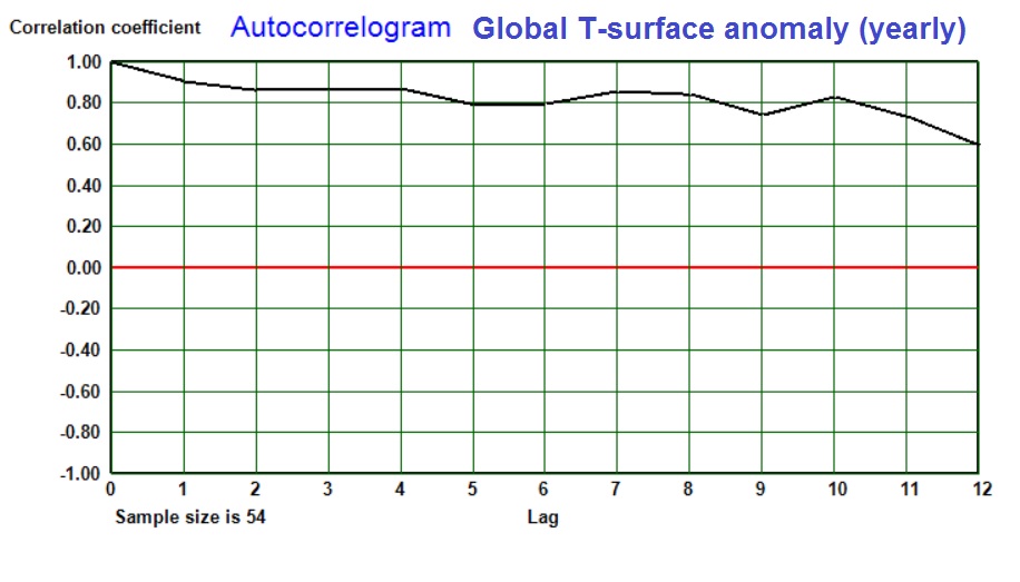
When analyzing a sequence of say, yearly data Y for randomness, it is useful to make regressions of Y on itself, where e.g. y(i) is correlated with y(i-1). Here a lag of one year is used, but larger lags are possible too, so that a Autocorrelogram can be drawn.This shows the "Auto Correlation Function (ACF). Often, the correlation coefficients are positive and gradually declining with increasing lag. Such condition may be called an "Auto Regressive" (AR) or "Auto Regressive Moving Average (ARMA) model". The global temperature anomaly, yearly averages, show strong autocorrelation as shown in the following autocorrelogram:
But the correlogram may show a wavy pattern, indicating cycles in the sequence of X. With the autocorrelated data in timeseries, the utmost care must be taken when interpreting the results of regressions. When considering the correlation of two time-series, all kinds of "spurious" correlation may occur (Fawcett, 2015). This means that very strong and significant correlations are found, but there is clearly no causal relationship!
The effect of autocorrelation is that the significance of correlations may be seriously overestimated. Autocorrelation means that the data in the series are not independent, but depend on the previous values. Hence the number of degrees of freedom (df) is overestimated. One remedy is to use the first differences of the values in each series. In the case of temperature above, the autocorrelation then disappears, and results become more informative. A correction of the number of degrees of freedom has been proposed by Bartlett(1946). This can reduce the df considerably:
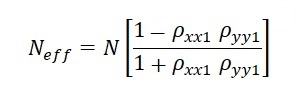
In the above formula (only one of a number of similar ideas), uses the product of the first order autocorrelation coefficient of X and Y. Here is an example of its use:

In view of the various correction formulas for the effective n, I tried also a formula which includes the sum of the autocorrelation matrix elements at all lags (as far as possible). Zieba (2010) and Bartels (1935). Applying this we get also an effective n of about 9, based on the first 6 lags.
Another way of correcting for autocorrelation is to calculate the "Partial Autocorrelation Function" (PACF). The , if lag 1 autocorrelation is predominant, we replace the data series with the estimates, using the PACF with lag 1, and subsequently by the residuals. In both the case of CO2 and Global T, this is sufficient for the correction. The a quite different regression result is obtained between, say, CO2 and Global T residuals, and vice versa. For instance there is a highly significant correlation between Global T and CO2at lag 1. and not at lag 2, Suggesting that Global T is the driver and increased CO2 the result after one year!
An interesting debate is wehther climate change has influenced homicide rates. Rather simple statistical investigations suggested that a warmer climate would enhance homicide rates. A more statistically correct investigation of a long record for New York and London showed no significant relationship, after correction for a.o. autocorrelation. (Lynch et al., 2020).
Autocorrelation can also occur along a borehole. Data derived from wireline logs will often show autocorrelation. A regression of porosity in samples on density may be seemingly more significant, or successful than the real relationship. A similar problem arises in trend analysis. I once studied the porosity in several wells in the Groningen gas field. A second degree trend surface had been calculated in order to predict porosity (dependent variable Z) for new well locations in the field. This involves the location coordinates X, Y, X2, Y2 and XY. The dependence of these "independent" variables tends to inflate the R-square (Coefficient of determination) and in false precision of the predicted porosity. Probably the best way to study autocorrelation in one- or two or more dimensions is kriging,, a system in which the autocorrelation is an advantage rather than a nuisance!
Causality?
An interesting way to study causality is the "Granger-causality", a method that establishes whether X values that precede Y have a significant effect on Y, as explained on Wikipedia. Although this method does not prove real causality, it supports a physical relationship between X and Y, if significant, even in the case of autocorrelation. So for the temperature anomaly (Hardcrut4) and CO2 series of the last 60 years (1959-2018) we see that Temperature (Granger)-causes a rise in CO2 a year later and a little two years later, while there is no influence of CO2 on temperature in this short time series.
With the various problems that may arise in a simple regression, it may help to apply cross-evaluation. This means, for example, that the regression is calculated on the first half of the data and Y estimated using the second half of the data, and vice versa. This usually shows that the prediction power of the regression equation is smaller than expected from the original result with all data pairs (see also the section on "predicted" R-square.
Another trick to obtain insight into the predictive value is the "Jacknife".
Relationships between variables can also be studied with other methods. Non-parametric correlation is sometimes useful and almost as powerful as the parametric method described above for linear correlation. For correlation important tools are "Rank correlation" of which at least two flavours exist: Kendall's tau (Kendall, 1970) and Spearman's rho (Spearman, 1904). The data are not required to be measured on an interval scale, only rank order. In Gaeapas a rank correlation is used in the analysis of variance, because of the nature of the data distributions involved. The rank correlations do not expect a linear relationship. If Y has a monotone, but non-linear relationship with X, it can give a significant result, which might be less significant for the Pearson correlation. But in general, the power to detect significant correlation is higher for the Pearson correlation coefficient. using a rank correlation is a trade-off between power and distribution-shape requirements.
Lag correlation is used when process in time creating the Y variable is influenced by the X variable from an earlier time. A interesting example is the gas production in the Groningen gas field, presumably causing earthquakes that cause multibillion Euros damage to houses and infrastructure, or loss of revenue in case production is reduced to mitigate the effect. Here changes in production level can be related to the number and intensity of the quakes, although the exact causal relationship is enormously complex and unsufficiently understood.
Having yearly data of production and numbers of eartquakes => 1.5 magnitude per year (1989 - 2017), a lag regression of this seismic activity on production gave the following results:
Rank correlation
Lag regression
Lag R-square d.f. Probability 0 0.1229 27 0.03115 * 1 0.2893 26 0.00158 ** 2 0.1927 25 0.01010 * 3 0.1363 24 0.03174 *
It seeems that the immediate seismic reaction to changes in production level is statistically significant at the 5% level, but too weak for prediction. By far the most important predictor appears to be the production changes in the year before. Earlier years also show statistical significance, but when a multiple regression is made with all the lags shown, the lag 1 is hardly trumped by the four lag combination. So we settle with the lag 1 correlation for prediction. Note that here any effect of autocorrelation, as discussed above, has not been taken into account.
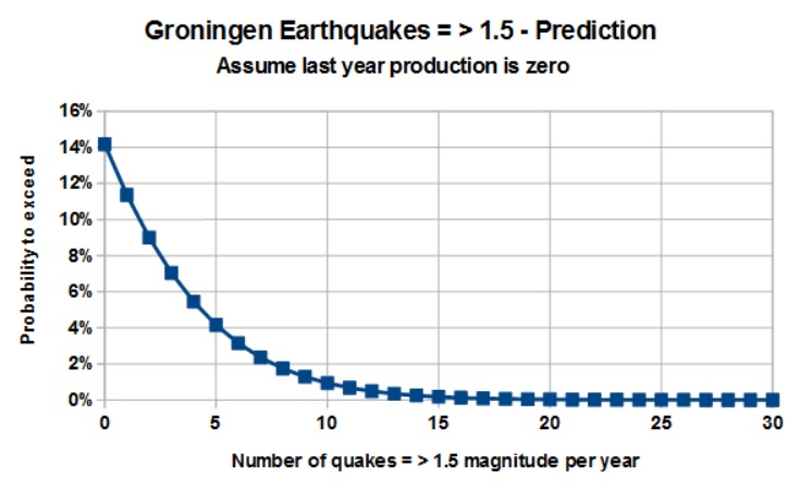
Two estimates are made: First, an expectation curve for earthquake frequency in 2018, based upon production in 2017, second, an expectation curve for, say, 2019, if production in 2018 is stopped completely. In both cases there is a still considerable chance of having a number of earthquakes = > 1.5 as shown in the graphs below, but the zero production suggests an important reduction.
A few caveats: There is strong autocorrelation in both production sequence and the seismic sequence. This has not been taken care of and affects the true numbers of freedom by inflation. And, the zero production is an extrapolation far below the minimum production in the dataset.
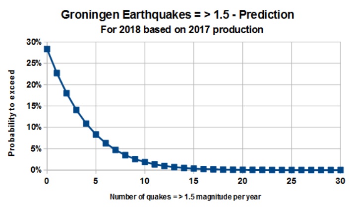
If the above analysis is sound, the results suggest that instead of maintaining the 2017 rate of production, zero production just about halves the probability of having a given number of earthquakes, compared to maintaining the 2017 level. But zero earthquakes requires zero production during several years. The effect of natural earthquakes has not been considered here.