Discovery Process Modeling - Creaming
Every study based only on the so-called proved reserves should be discarded as useless following
the principle GIGO: Garbage In, Garbage Out.
Laherre, 2006
A discovery process model
- One-dimensional Creaming
- Four-dimensional creaming
- Growth of Ultimate Recovery
- Estimating the number of future discoveries
The first linear model of exploration and production was a logistic growth curve used successfully by M.K.Hubbert in 1956, projecting the peak of conventional oil discovery and production in the US. In 1973, FitzPatrick, et al, made estimates on the basis of the Gompertz curve and simpeler derived models. Later, for similar models, the term "creaming" (short for "creaming off") was coined in Shell Intnl. in the seventies when the work of Arps and Roberts (1958) and Drew (1974) became known. The idea is that the exploration process in a basin "creams off" the best prospects first, gradually having to consider more risky prospects. One could imagine that the large anticlines are so conspicuous that they are easier to find than the smaller more subtle closures. After that, fault traps against one fault and eventually more risky traps bounded by several faults would be drilled. In reality the process will be less organized, but in many basins the general trend is obvious.
There are various graphs that can be made to show the discovery process:
- Cumulative volume discovered vs years on the horizontal axis.
- Cumulative volume discovered vs number of exploration wells
- Cumulative number of discoveries vs number of exploration wells (slope is success rate).
This type of analysis of the discovery process is "one-dimensional" as it involves one independent variable: exploration effort in terms number of wildcats, or also sometimes just time in years.
From a statistical point of view, the exploration process is a sampling without replacement from a finite population of exploration prospects. Without geology and geophysics this sampling may be random. However, even if the basin is drilled at random locations, the prospects with a larger 2-dimensional size have a slightly better chance to be found first. So even in that theoretical case there would be some creaming effect. The bias in the sampling will be still larger if geological insight, seismic and other surveys and geochemistry become involved. As the prospects portfolio becomes depleted we see that both the mean of and the variance of the population of the remaining prospects are decreasing.
Here is an example of cumulative discovery vs. cumulative number of exploration wells:
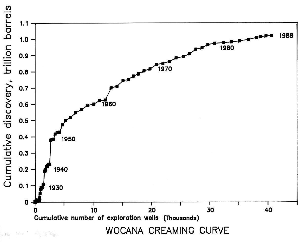
The part of the globe represented by this graph is "World Outside Communist Areas and North America". It is outdated in two respects: it was made in 1989 and the ultimate recoveries of the field discovered in say the last ten years of the graph will have changed. Nevertheless, there is considerable creaming.
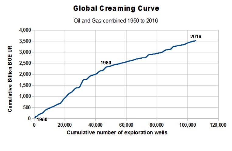
In a recent article by E.Smith Llim�s (2017) in the AAPG Explorer, a graph of yearly number of new Field Wildcats drilled and yearly discovery of conventional oil and gas in terms of barrels oil equivalent (BOE). It shows that since 2008, both drilling and discovery volume has declined considerably, suggesting a rather gloomy situation for conventional oil and gas, which is true, of course, with regard to the exploration activity. However, both declines are mainly influenced by economics at low oilprices, not geology! To show this I used the data extracted from the graph to construct a creaming curve of cumulative discovery versus cumulative exploration wells. This shows that the success rate in terms of BOE was high before 1980, and a little less since then, but there is no suggestion at all for a decline in recent decades. A good example to stress the importnace to work with exploration effort instead of years.
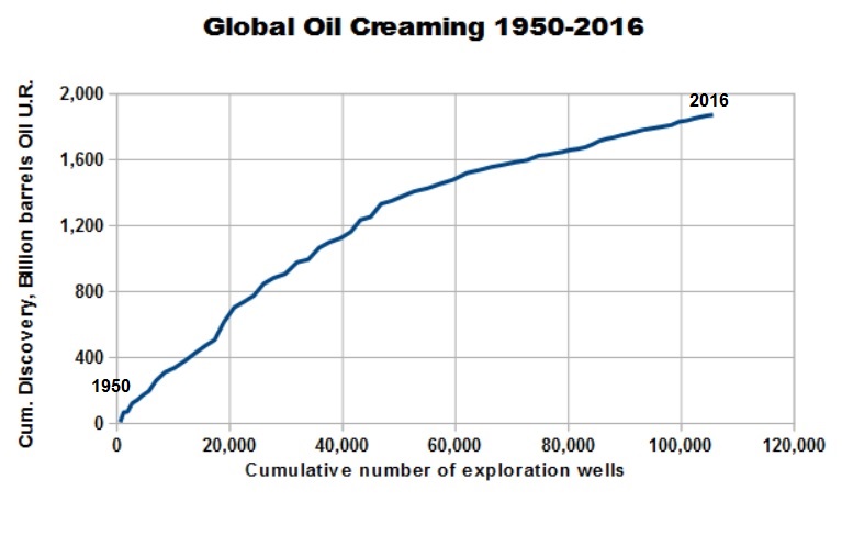
The data allow even a split into the amounts of oil and gas discovery separately, so the oil and gas creaming curves are as shown below. Both show no decline in discovery rate since 1980.
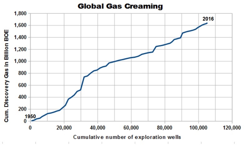
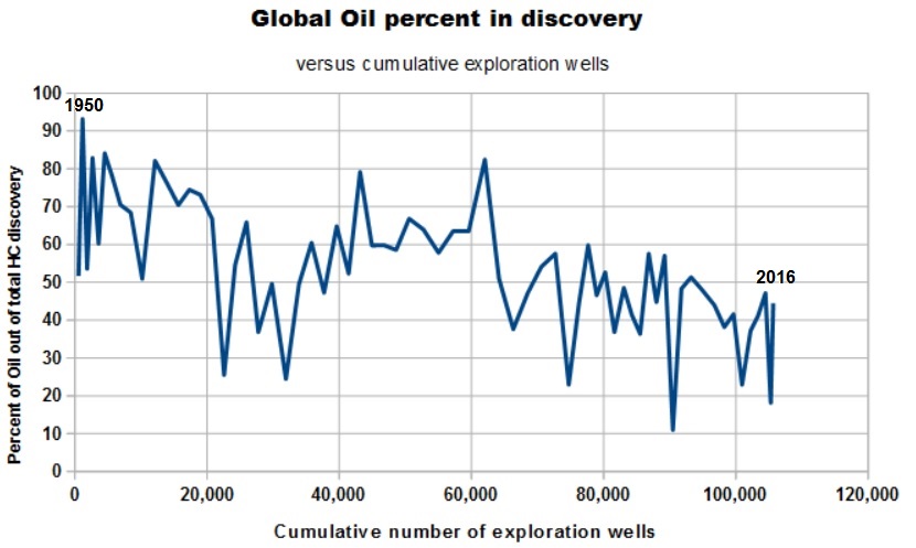
An important change is that in this period a significant change occurs from oil to gas as the predominant HC found. This is shown by the percentage of oil in the HC mix discovered, here against the cumulative number of wells, but a similar picture is obtained if we simply put years at the X-axis.
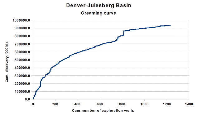
The "classic" creaming curve is from the Denver-Julesberg basin, cum. discovery up to a billion barrels against cum. number of exploration wells:
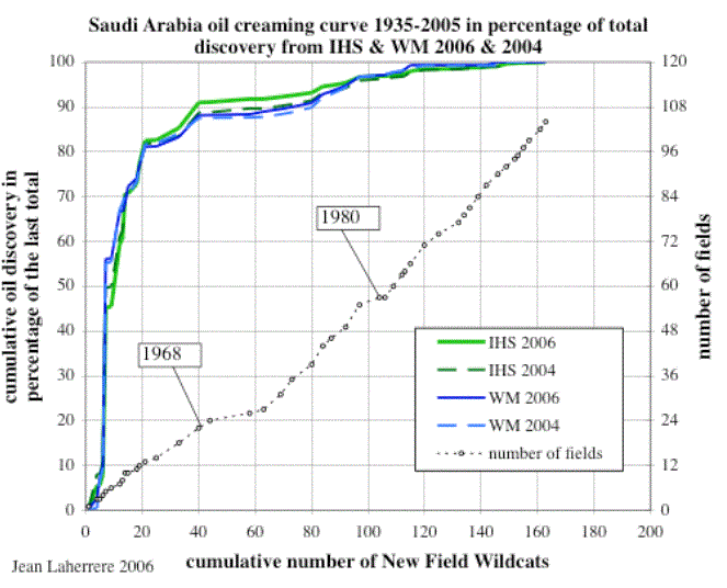
Various attempts to make extrapolations for forecasting have been made over the years, e.g. Meisner & Demirmen (1981) have developed a bayesian approach to creaming. I used this for a forecast of UK offshore production made in the early 80ies by UKOOA. Extrapolation of the creaming process allowed a probabilistic estimate of the undiscovered fields.
For a single field, the updates of the UR over the year may present an erratic behavior. More interesting and useful is to obtain data for a set of fields, say 10 or 20. The the UR data and years of the fields are shifted to a common date. The sums of the year columns give the UR history for the total set of fields. These numbers divided by the initial UR are the CGF values. A regression of log(CGF) on Log(year) provides an estimate of the above mentioned constants.
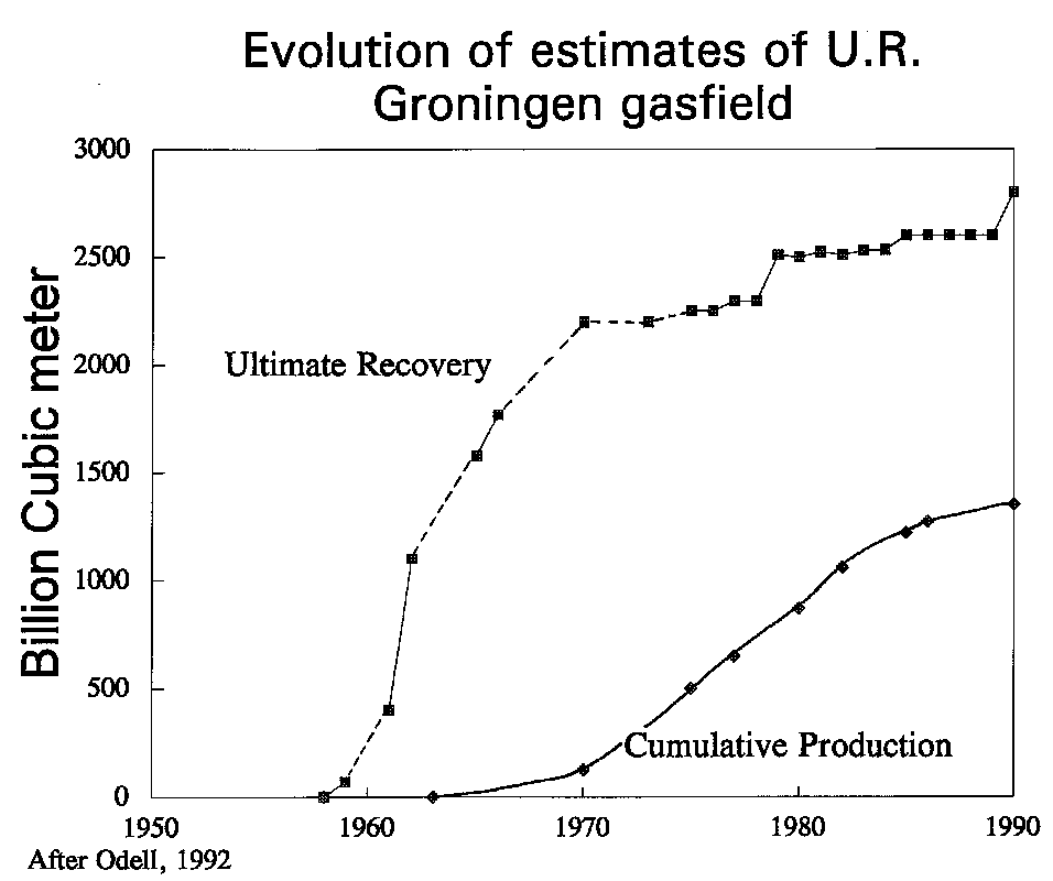
In a study of field reserves of some 600 fields outside the USA in 1985, I found a growth factor of over two after 7 years. From year zero to year seven the increase was roughly linear. Of course, this growth is the average of many fields. Some are initially overestimated, others underestimated. However, underestimation is the rule. Especially if reserve data refer to "proven" reserves (P90), just because data on Ultimate Recovery are not available, the chances of growth are high. An extreme example of U.R. growth is the Groningen gas field in the Netherlands:
Other examples of the revision of Ultimate Recovery estimates are given for UK and Norway by Hermanrud et al. (1996), Dromgoole et al. (1997) and Chengliu et al. (2014). An excellent and readily available paper is by Crovelli and Schmoker (1998) and a good source for further reading.
Significant growth means that a reserves creaming needs correction to the last, say ten years, otherwise the creaming process will severely underestimate the undiscovered reserves as well. However, the advances in seismic techniques and coverage by 3D have made the initial estimates for the more recent fields much less biased.
The growth of reserves means that for a proper creaming analysis, it is essential to assign the "rolled-back" U.R. to the discovery year, otherwise the strength of the creaming process might be underestimated.
The definition of the province, basin, or play that is analysed is very important. Each subdivision may have its own creaming curve. For instance, technical limitations have prevented deepwater exploration in earlier days. Also maximum depth of exploration plays a role. Then gradually prolific areas become available later, partly because of technical reasons. Especially creaming against a time scale rather than against number of exploration wells would become unreliable. So, areas for creaming have to be defined carefully on the basis of both geological and technical grounds.Estimating the number of discoveries that can be made in a play
When a play has n prospects, each with its own ,POS, it is fairly easy to obtain a distribution of the number of successes if we drill all the prospects. The procedure uses the binomial distribution not with a single fixed probability, but the various POS values for the prospects. For n < 14 it is possible to enumerate all possible permutations and extract the distribution of numbers of discoveries. The logic becomes clear if we use an example of only 3 prospects. Then the number of possibilities is 2^3 = 8 (and , in general 2^n). The 8 possible combinations are listed in the 8 rows in the left three columns of the table. The last two columns show the resulting number of discoveries for each cobination and the probability that a combination will occur.
| Prospect 1 | Prospect 2 | Prospect 3 | Number of discoveries | Probability |
|---|---|---|---|---|
| POS = 0.35 | POS = 0.12 | POS = 0.55 | ||
| 0 | 0 | 0 | 0 | 0.2574 |
| 1 | 0 | 0 | 1 | 0.1386 |
| 0 | 1 | 0 | 1 | 0.0351 |
| 0 | 0 | 1 | 1 | 0.3146 |
| 1 | 1 | 0 | 2 | 0.0189 |
| 1 | 0 | 1 | 2 | 0.1694 |
| 0 | 1 | 1 | 2 | 0.0429 |
| 1 | 1 | 1 | 3 | 0.0231 |
| SUM = | 1.0000 |
The probabilities are derived by multiplication ( this assumes independence of the prospects). For instance, In the first permutation, only prospect 1 is a success (indicated by a "1"). The probability of this result from three prospects drilled is p1 * (1- p2) * (1 - p3) = 0.35 * (1 - 0.12) * (1 - 0.55) = 0.2574.
Now by assembling the probabilities for 0,1, 2 and 3 discoveries we get:
| Number of discoveries | Probability |
|---|---|
| 0 | 0.2574 |
| 1 | 0.4883 |
| 2 | 0.2312 |
| 3 | 0.0231 |
For larger n an approximation based on the normal distribution can be used, then based on the average of the prospect probabilities.
This analysis of probabilities also plays a role in hindsight analysis of prospect appraisals.